Source transformation is a technique used to simplify circuits by converting between equivalent voltage sources and current sources. Although this article explains source transformation using resistive circuits, the same idea can later be applied to circuit analysis involving phasors or the Laplace transform. Source transformation is one of the fundamental circuit analysis methods for obtaining an equivalent circuit when viewed from a specific point, and it provides an intuitive way to understand and analyze circuits.

Mutual Conversion Between Current Sources and Voltage Sources

The internal resistance of a voltage source approaches ideal behavior as it gets closer to 0, while the internal resistance of a current source approaches ideal behavior as it gets closer to \(\infty\). In real-world circuits, the internal resistance of a source has a meaningful, measurable value. This non-ideality is commonly modeled by representing a voltage source as an ideal voltage source in series with a resistor, and a current source as an ideal current source in parallel with a resistor. These internal resistances can be combined with surrounding resistors in series or parallel during circuit analysis. In general, the resistors directly related to a voltage source’s internal resistance are those connected in series with the source, while the resistors directly related to a current source’s internal resistance are those connected in parallel with the source.

Source transformation essentially refers to the equivalent conversion between a voltage source and a current source. It simplifies a circuit by converting a voltage source with a series resistor into a current source with a parallel resistor, or vice versa. The circuit in form (A) of Fig. 1 can be transformed into form (B), and conversely, the circuit in form (B) can be transformed into form (A).

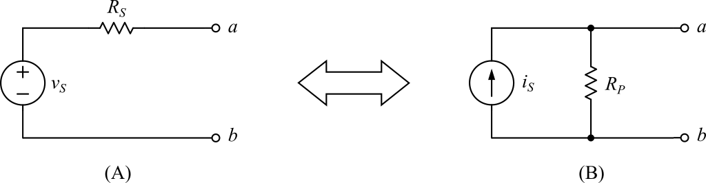
Let us examine the internal resistance seen from terminals a and b for cases (A) and (B) in Fig. 1. In circuit (A), since \(v_S\) is an ideal voltage source with zero internal resistance, it can be considered a short circuit. Viewed from terminals a and b, only \(R_S\) appears as the internal resistance. In circuit (B), since \(i_S\) is an ideal current source with infinite internal resistance, it can be considered an open circuit. Viewed from terminals a and b, only \(R_P\) appears as the internal resistance. Because circuits (A) and (B) are equivalent when viewed from terminals a and b, their internal resistances must be equal. Therefore, the following relationship must hold.

\[R_S = R_P\tag{1.1}\label{eq:r_eq}\]

Next, consider the open-circuit voltage \(V_{ab}\) between terminals a and b when nothing is connected to them in circuits (A) and (B). Since (A) and (B) are interchangeable equivalent circuits, this open-circuit voltage \(V_{ab}\) must also be the same for both. For circuit (A),

\[V_{ab} = v_S\tag{1.2}\label{eq:ov_a}\]

can be obtained immediately. For circuit (B), the voltage across terminals a and b is caused by the source current \(i_S\) flowing through \(R_P\). By Ohm’s law,

\[V_{ab} = i_S R_P\tag{1.3}\label{eq:ov_b}\]

From equations (\ref{eq:ov_a}) and (\ref{eq:ov_b}), the following relationship between equivalent circuits (A) and (B) can be obtained.

\[v_S = i_S R_P\tag{1.4}\label{eq:st_eq1}\]

Now, consider an extreme load condition where terminals a and b are shorted. If circuits (A) and (B) are truly equivalent, the current \(I_{ab}\) flowing through the short between terminals a and b must be the same. In circuit (A), when terminals a and b are shorted, the current flowing through them is, by Ohm’s law,

\[I_{ab}=\frac{v_S}{R_S}\tag{1.5}\label{eq:oi_a}\]

In circuit (B), all of the source current \(i_S\) flows into the shorted terminals a and b, so

\[I_{ab} = i_S\tag{1.6}\label{eq:oi_b}\]

follows directly. By rearranging equations (\ref{eq:oi_a}) and (\ref{eq:oi_b}), another relationship between equivalent circuits (A) and (B) is obtained.

\[i_S = \frac{v_S}{R_S}\tag{1.7}\label{eq:st_eq2}\]

Finally, by combining equations (\ref{eq:r_eq}), (\ref{eq:st_eq1}), and (\ref{eq:st_eq2}), the formulas used for source transformation can be summarized as follows.

Example of Circuit Application

Suppose we want to calculate the power supplied from the \(10V\) source on the left to the rest of the circuit in circuit (1) of Fig. 2. To do so, it is convenient to simplify the rest of the circuit as much as possible. First, the \(5\Omega\) resistor connected in series with the \(20V\) source on the far right of circuit (1) can be transformed into a current source with a \(5\Omega\) resistor in parallel using equation (\ref{eq:st_form}). The \(5\Omega\) resistor is connected in parallel without change, and the value of the current source becomes

\[i_S = \frac{v_S}{R_S} = \frac{20}{5} = 4\enspace(A)\]

Thus, the circuit can be redrawn as circuit (2) in Fig. 2. In circuit (2), the equivalent resistance of the \(20\Omega\) and \(5\Omega\) resistors connected in parallel with the \(4A\) current source is \(20||5 = 4\Omega\). Applying source transformation again, this can be converted into a voltage source with a \(4\Omega\) series resistor. Using equation (\ref{eq:st_form}), the voltage source value is

\[v_S = i_S R_S = 4 \cdot 4 = 16\enspace(V)\]

Using this result, the circuit can be redrawn as circuit (3) in Fig. 2.

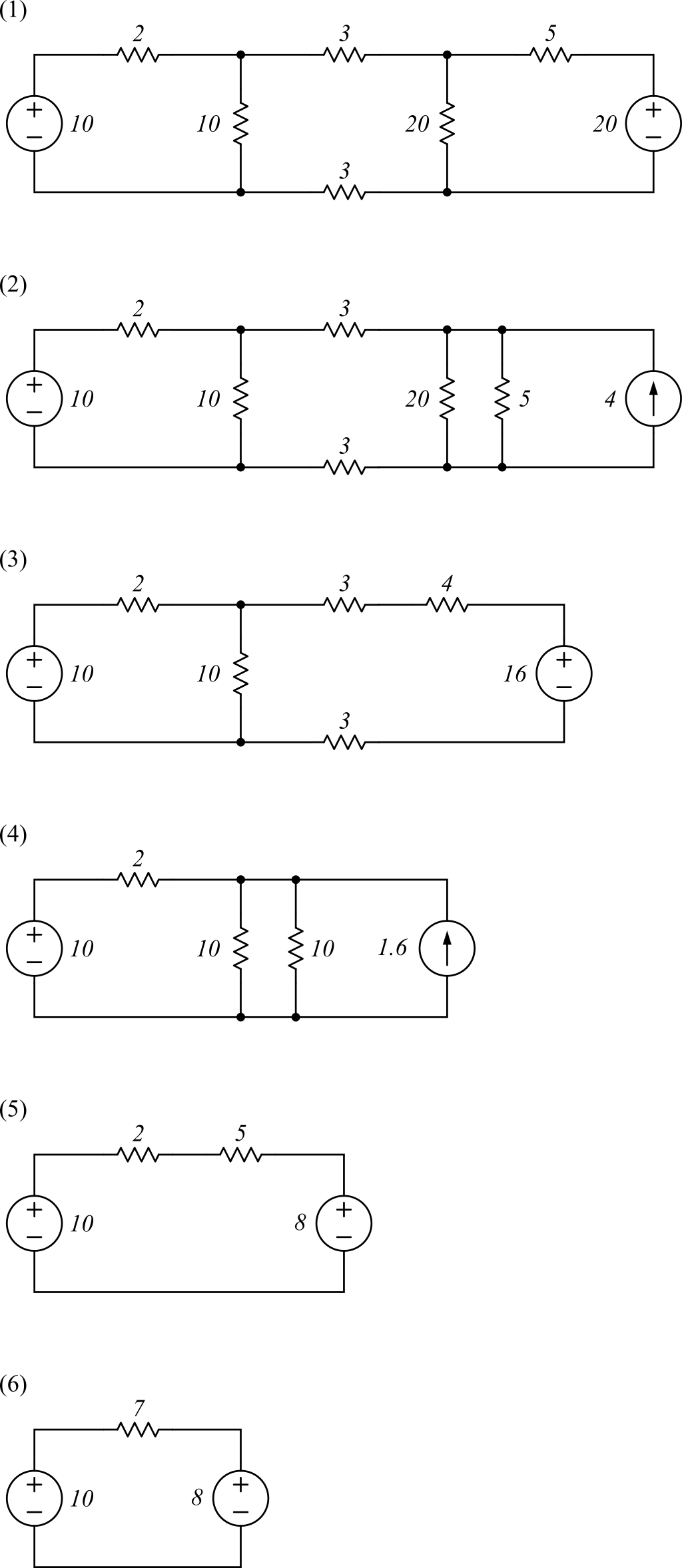
In circuit (3), the total resistance in series with the \(16V\) voltage source is \(3 + 4 + 3 = 10\Omega\). This can again be transformed into a current source with a \(10\Omega\) resistor in parallel.

\[i_S = \frac{v_S}{R_S} = \frac{16}{10} = 1.6\enspace(A)\]

Redrawing the circuit using the calculated \(1.6A\) current source and the \(10\Omega\) parallel resistor yields circuit (4) in Fig. 2. In circuit (4), the equivalent resistance of the two \(10\Omega\) resistors connected in parallel is \(5\Omega\). This can again be transformed into a voltage source with a \(5\Omega\) series resistor.

\[v_S = i_S R_S = 1.6 \cdot 5 = 8\enspace(V)\]

Using this result, the circuit can be simplified and redrawn as circuit (5) in Fig. 2. The series resistance in circuit (5) is \(2 + 5 = 7\Omega\), so the circuit is finally reduced to circuit (6).

Finally, in the simplified circuit (6) of Fig. 2, the power supplied from the \(10V\) source to the circuit can be calculated very easily. First, using KVL, the current \(i_S\) flowing from the \(10V\) source toward the \(7\Omega\) resistor is calculated as

\begin{align} 10 - 7i_S -8 &= 0 \\ 7i_S &= 2 \\ i_S &= \frac{2}{7}\enspace(A) \end{align}

As a result, the power supplied by the \(10V\) source to the circuit is calculated as

\[p = v_S \cdot i_S = 10 \cdot \frac{2}{7} \approx 2.86\enspace{W}\]

Conclusion

Source transformation is a technique for simplifying a circuit by determining an equivalent circuit as seen from a specific point. Although it is a basic analysis method that applies only to circuits composed of independent voltage or current sources and linear elements, it forms the theoretical foundation for understanding Thevenin and Norton equivalents introduced later. By fully understanding that a voltage source with a series resistor and a current source with a parallel resistor are equivalent and interchangeable through simple calculations, one can develop stronger intuition for future circuit analysis.