This article introduces the Node Voltage Method (NVM) and the Mesh Current Method (MCM). These two circuit analysis techniques are based on the most fundamental principles in circuit theory: Kirchhoff’s Current Law (KCL) and Kirchhoff’s Voltage Law (KVL). To explain these methods, we will focus on resistive circuits that only include resistors, independent sources, and dependent sources. Both the node voltage and mesh current methods described here are applicable even in more advanced analysis techniques such as phasor analysis and Laplace transforms. Therefore, it is fair to say that these are one of the most fundamental and essential techniques for circuit analysis.

Prerequisite Knowledge

Voltage

Voltage is the difference in electric potential energy between two points. It is commonly defined as the energy per unit charge. Simply put, a higher voltage implies that more electrical energy is present. If there is no voltage difference, then charge will not move, and therefore, no current will flow.

\[\begin{align*} v &= \frac{dw}{dq} \\ \\ where&\\ \quad v&=voltage\ (Volts,\ V) \\ \quad w&=energy\ (Joules,\ J) \\ \quad q&=charge\ (Coulombs,\ C) \\ \end{align*}\]

Current

Current is the flow of electric charge. Mathematically, it is defined as the amount of charge that flows per unit time. In other words, if more charge moves in a given time interval, the current is greater.

\(\begin{align*} i &= \frac{dq}{dt} \\ \\ where&\\ \quad i&=current\ (Amperes,\ A) \\ \quad q&=charge\ (Coulombs,\ C) \\ \quad t&=time\ (Seconds,\ sec) \\ \end{align*}\)

Ohm's law

Ohm’s Law states that the voltage between any two points in a conductor is directly proportional to the current flowing through it, and also to the resistance between those two points. This relationship is expressed by the following formula:

\(\begin{equation} V = I\cdot R \tag{1.1} \label{eq:ohms_law} \end{equation}\)

Rearranging Equation~(\ref{eq:ohms_law}) with respect to \(I\) or \(R\) gives:

\[\begin{equation} I = \frac{V}{R}\quad or\quad R = \frac{V}{I} \tag{1.2} \label{eq:ohms_law_altered} \end{equation}\]

These alternate forms of Ohm's Law offer different perspectives. The first shows that for the same amount of current, a larger resistance causes a greater voltage drop across the resistor. Alternatively, for a constant voltage, increasing the resistance reduces the current. The second expression shows that resistance \(R\) is essentially a proportionality constant between voltage and current.

Kirchhoff's Current Law (KCL)

Kirchhoff’s Current Law states that the sum of all currents entering a node must equal the sum of all currents leaving that node. This is essentially a law of current conservation. If we treat outgoing currents as positive and incoming currents as negative, the algebraic sum of all currents connected to a node is always zero:

 

\[\begin{equation*} \sum_{k=1}^{n} I_k = 0 \end{equation*}\]

Kirchhoff's Voltage Law (KVL)

Kirchhoff’s Voltage Law states that the algebraic sum of the voltage changes around any closed loop in a circuit is zero. That is, if you trace around a loop starting from any point and return to the same point, the net change in voltage is zero. Voltage increases are treated as positive, and drops as negative:

\begin{equation*} \sum_{k=1}^{n} V_k = 0 \end{equation*}

Voltage Divider

When a voltage is applied across resistors connected in series, each resistor receives a portion of the total voltage proportional to its resistance. Such a circuit configuration is called a voltage divider.

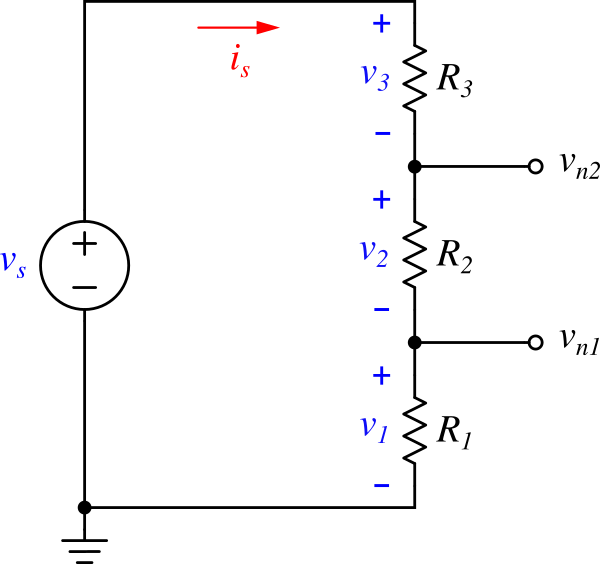
Figure 1: Voltage divider example

Figure 1 shows a voltage divider circuit composed of three resistors. These resistors divide the total voltage \( v_s \) into \( v_1 \), \( v_2 \), and \( v_3 \), each receiving a share according to its resistance. To compute these voltages, let’s apply Kirchhoff’s Voltage Law (KVL) to the circuit.

Now, let's apply KVL to Figure 1. There is only one loop, so there's no choice needed. Let the current be \( i_s \), and assume it flows clockwise. We'll choose the ground at the bottom left as the starting point. Note that the direction of the loop and the starting point do not affect the final result. As we go around the loop starting from the ground node, we first encounter the independent voltage source, which increases the potential by \( v_s \), so this contributes \( +v_s \). Then, as we pass through each of the three resistors, the voltage drops by \( v_1 \), \( v_2 \), and \( v_3 \), respectively. Adding all these voltage changes and setting their sum to zero gives the following KVL equation:

\begin{equation} v_s - v_3 - v_2 - v_1 = 0 \tag{1.3} \label{eq:vdiv_kvl} \end{equation}

Rearranging Equation~(\ref{eq:vdiv_kvl}) in terms of \( v_s \), substituting each voltage using Ohm’s Law, and relating the result to \( v_s = i_s R_{eq} \), we get:

\begin{align} v_s &= v_1 + v_2 + v_3 \nonumber\\ &= i_s R_1 + i_s R_2 + i_s R_3 \nonumber\\ &= i_s(R_1 + R_2 + R_3) \nonumber\\ &= i_s R_{eq} \tag{1.4} \label{eq:vdiv_kvl_} \end{align}

From Equation~(\ref{eq:vdiv_kvl_}), we obtain the relationship for the equivalent resistance \( R_{eq} \) of resistors \( R_1, R_2, R_3 \) connected in series. This tells us that the equivalent resistance is simply the sum of all individual resistances:

\begin{equation*} R_{eq} = R_1 + R_2 + R_3 \end{equation*}

This equation can be generalized for \( k \) resistors connected in series as follows:

Rewriting Equation~(\ref{eq:vdiv_kvl_}) in terms of \( i_s \), we get:

\begin{equation} i_s = \frac{v_s}{R_1 + R_2 + R_3} = \frac{v_s}{R_{eq}} \tag{1.5} \label{eq:vdiv_is} \end{equation}

The voltage across each resistor can be found using Ohm's Law: \( v_1 = i_s R_1 \), \( v_2 = i_s R_2 \), \( v_3 = i_s R_3 \). Substituting \( i_s \) from Equation~(\ref{eq:vdiv_is}), we obtain:

\begin{align} v_1 &= i_s R_1 = \frac{v_s}{R_{eq}}R_1 = \frac{R_1}{R_1 + R_2 +R_3}v_s \nonumber \\ v_2 &= i_s R_2 = \frac{v_s}{R_{eq}}R_2 = \frac{R_2}{R_1 + R_2 +R_3}v_s \nonumber \\ v_3 &= i_s R_3 = \frac{v_s}{R_{eq}}R_3 = \frac{R_3}{R_1 + R_2 +R_3}v_s \tag{1.6} \label{eq:vdiv_ratio} \end{align}

Equation~(\ref{eq:vdiv_ratio}) demonstrates that the voltage across each resistor is proportional to its resistance. It also shows that the ratio between each resistor’s voltage and the total voltage \( v_s \) equals the ratio between that resistor’s value and the total equivalent resistance \( R_{eq} \).

 

Finally, the terminal voltages \( v_{n1} \) and \( v_{n2} \) shown in Figure 1 are:

\begin{align*} v_{n1} &= v_1 = \frac{R_1}{R_1 + R_2 +R_3}v_s \\ v_{n2} &= v_1 + v_2 = \frac{R_1 + R_2}{R_1 + R_2 + R_3}v_s \end{align*}

 

Current Divider

In resistors connected in parallel, the current flowing through each branch is inversely proportional to the resistance of that branch. In other words, a branch with higher resistance draws less current, while a branch with lower resistance draws more current.

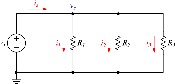
Figure 2: Current divider example

In Figure 2, the three resistors \( R_1 \), \( R_2 \), and \( R_3 \) are connected in parallel to an independent voltage source \( v_s \). This parallel resistor network is also called a current divider. By applying Kirchhoff’s Current Law (KCL) at the \( v_s \) node, we can derive the current relationship for each branch.

In Figure 2, the voltage at node \( v_s \) is determined by the independent voltage source. The branch currents are shown in red in the diagram. Applying KCL at the \( v_s \) node, we sum all currents: \( i_s \) flows into the node, so it is assigned a negative sign, while \( i_1 \), \( i_2 \), and \( i_3 \) flow out of the node and are assigned positive signs. Summing all of them and setting the total to zero gives the following KCL equation:

\begin{equation} -i_s + i_1 + i_2 + i_3 = 0 \tag{1.7} \label{eq:cdiv_kcl} \end{equation}

Applying Ohm’s Law to \( i_1 \), \( i_2 \), and \( i_3 \) in Equation~(\ref{eq:cdiv_kcl}) gives:

\begin{align} i_1 &= \frac{v_s}{R_1}\nonumber\\ i_2 &= \frac{v_s}{R_2}\nonumber \\ i_3 &= \frac{v_s}{R_3} \tag{1.8} \label{eq:cdiv_bcur} \end{align}

Substituting (\ref{eq:cdiv_bcur}) into (\ref{eq:cdiv_kcl}) and using the relationship \( i_s = \frac{v_s}{R_{eq}} \), we get:

\begin{align*} i_s &= \frac{v_s}{R_1} + \frac{v_s}{R_2} + \frac{v_s}{R_3}\nonumber\\ &= \left(\frac{1}{R_1}+\frac{1}{R_2}+\frac{1}{R_3}\right)v_s\nonumber\\ &=\frac{1}{R_{eq}} v_s \tag{1.9} \label{eq:cdiv_drv} \end{align*}

From Equation~(\ref{eq:cdiv_drv}), we can derive the expression for the equivalent resistance of parallel resistors:

\begin{equation*} \frac{1}{R_{eq}} = \frac{1}{R_1} + \frac{1}{R_2} + \frac{1}{R_3} \end{equation*}

This formula can be generalized for \( k \) parallel resistors as follows:

Finally, using Ohm’s Law to replace \( v_s \) in Equation~(\ref{eq:cdiv_bcur}) with \( R_{eq} i_s \), we get:

\begin{align} i_1 &= \frac{v_s}{R_1} = \frac{R_{eq}}{R_1} i_s \nonumber\\ i_2 &= \frac{v_s}{R_2} = \frac{R_{eq}}{R_2} i_s \nonumber\\ i_3 &= \frac{v_s}{R_3} = \frac{R_{eq}}{R_3} i_s \\ & \text{where, } R_{eq} = \frac{R_1 R_2 R_3}{R_1R_2 + R_2R_3 + R_1R_3} \nonumber \tag{1.10} \label{eq:cdiv_result} \end{align}

Equation~(\ref{eq:cdiv_result}) shows that the current through each resistor in a current divider is inversely proportional to its resistance. It also confirms that the ratio of current through each resistor to the total current \( i_s \) equals the ratio of the equivalent resistance to the resistance of that branch.

Node Voltage Method (NVM)

The Node Voltage Method (NVM), also known as nodal analysis, is a circuit analysis method that calculates the voltage at each node by applying Kirchhoff’s Current Law (KCL).

Let’s apply NVM to a few examples.

NVM Example with Independent Sources Only

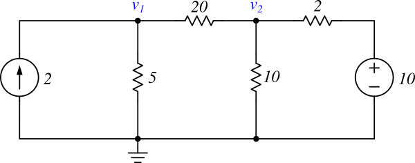
Figure 3: NVM example circuit with independent sources

Figure 3 shows a resistive circuit that includes only independent sources. There are two nodes with unknown voltages, which we label as \( v_1 \) and \( v_2 \), and mark in blue. For simplicity, units are omitted (assume standard SI units for resistance, voltage, and current). The GND node is the reference, and its voltage is always zero.

First, apply KCL at node \( v_1 \). This node connects to three branches:

• A 2A independent source injects 2A into the node → \(-2\)
• Through the \(5\Omega\) resistor: \( \frac{v_1}{5} \)
• Through the \(20\Omega\) resistor (from \(v_1\) to \(v_2\)): \( \frac{v_1 - v_2}{20} \)

Summing these currents and setting to zero gives:

\begin{equation} -2+\frac{v_1}{5}+\frac{v_1 - v_2}{20} = 0 \tag{2.1} \label{eq:ex1_kcl1} \end{equation}

Now apply KCL at node \( v_2 \). The three currents flowing out through \(20\Omega\), \(10\Omega\), and \(2\Omega\) resistors are:

• \( \frac{v_2 - v_1}{20} \)
• \( \frac{v_2}{10} \)
• \( \frac{v_2 - 10}{2} \)

Adding them and setting to zero gives:

\begin{equation} \frac{v_2 - v_1}{20} + \frac{v_2}{10} + \frac{v_2 - 10}{2} = 0 \tag{2.2} \label{eq:ex1_kcl2} \end{equation}

Combining equations~(\ref{eq:ex1_kcl1}) and (\ref{eq:ex1_kcl2}), we obtain the following system of equations:

\begin{alignat}{3} 5v_1 &&-v_2 = &&40 \nonumber\\ -v_1 &&+13v_2 = &&100 \tag{2.3} \label{eq:ex1_simul} \end{alignat}

Solving this system~(\ref{eq:ex1_simul}) gives the node voltages \( v_1 \) and \( v_2 \). In this article, we solve this normalized system using Cramer’s Rule. First, compute the determinant of the coefficient matrix:

\begin{equation*} \Delta = \left| \begin{array}{rr} 5 & -1 \\ -1 & 13 \end{array} \right| = 5 \cdot 13 -1 = 64 \end{equation*}

Now compute \( v_1 \) and \( v_2 \) using Cramer’s Rule:

\begin{equation*} \begin{split} v_1 &= \frac{1}{\Delta} \left| \begin{array} {rr} 40 & -1 \\ 100 & 13 \end{array} \right| \\ &= \frac{1}{64} (40 \cdot 13 - (-1) \cdot 100) \\ &\approx 9.69\ (V) \\[10pt] v_2 &= \frac{1}{\Delta} \left| \begin{array}{rr} 5 & 40 \\ -1 & 100 \end{array} \right| \\ &= \frac{1}{64} (5\cdot 100-40 \cdot (-1)) \\ &\approx 8.44\ (V) \end{split} \end{equation*}

Now that the node voltages are known, branch currents can easily be computed. For example, the current flowing through the \(20\Omega\) resistor from \(v_1\) to \(v_2\) is:

\begin{equation*} \frac{v_2 - v_1}{20} = \left(\frac{8.44 - 9.69}{20}\right) = -62.5\ (mA) \end{equation*}

Here, the negative current \( -62.5 \text{ mA} \) flowing from \( v_1 \) to \( v_2 \) actually means a positive current of \( 62.5 \text{ mA} \) flows from \( v_2 \) to \( v_1 \).

NVM with Dependent Sources

When a circuit includes a dependent source, an additional unknown variable is introduced, which results in an extra equation. Aside from this minor addition, the basic application of NVM remains the same.

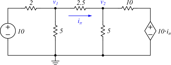
Figure 4: NVM example circuit with a dependent source

Figure 4 shows a resistive circuit that includes a current-controlled voltage source (CCVS). The control variable of the CCVS, \( i_\pi \), is the current flowing through the \( 2.5\Omega \) resistor (as shown with a blue arrow in the diagram). According to Ohm's Law, \( i_\pi \) can be written as:

\begin{equation} i_\pi = \frac{v_1 - v_2}{2.5} \tag{2.4} \label{eq:ex2_dep_var} \end{equation}

Now we apply NVM by writing KCL equations at each node and then solve the resulting system using the expression for \( i_\pi \). First, the KCL equation at node \( v_1 \) is:

\begin{equation} \frac{v_1 - 10}{2} + \frac{v_1}{5} + i_\pi = 0 \tag{2.5} \label{eq:ex2_kcl1} \end{equation}

Then, the KCL equation at node \( v_2 \) is:

\begin{equation} -i_\pi + \frac{v_2}{5} + \frac{v_2 -10i_\pi}{10} = 0 \tag{2.6} \label{eq:ex2_kcl2} \end{equation}

By substituting Equation~(\ref{eq:ex2_dep_var}) into both (\ref{eq:ex2_kcl1}) and (\ref{eq:ex2_kcl2}), we eliminate \( i_\pi \) and obtain the following system of equations:

\begin{alignat}{3} 11v_1 &&-4v_2 = &&\ 50 \nonumber\\ -8v_1 &&+11v_2 = &&\ 0 \tag{2.7} \label{eq:ex2_simul} \end{alignat}

Using Cramer’s Rule, we now solve the system~(\ref{eq:ex2_simul}) to find \( v_1 \) and \( v_2 \). First, the determinant of the coefficient matrix \( \Delta \) is:

\begin{equation*} \Delta = \left| \begin{array}{rr} 11 & -4 \\ -8 & 11 \end{array} \right| =11 \cdot 11 - (-4)\cdot(-8) = 89 \end{equation*}

Now calculate \( v_1 \) and \( v_2 \) as follows:

\begin{align*} v_1 &= \frac{1}{\Delta} \left| \begin{array}{rr} 50 & -4 \\ 0 & 11 \end{array} \right| \\ &=\frac{1}{89}(50 \cdot 11 - (-4)\cdot 0) \\ &\approx 6.18\ (V) \\[10pt] v_2 &= \frac{1}{\Delta} \left| \begin{array}{rr} 11 & 50 \\ -8 & 0 \end{array} \right|\\ &=\frac{1}{89}(11 \cdot 0 - 50 \cdot (-8))\\ &\approx 4.49\ (V) \end{align*}

Supernode

When two nodes in a circuit are connected by an ideal voltage source, they can be treated as a single node when applying KCL. This combined node is called a supernode. Let's examine a concrete example.

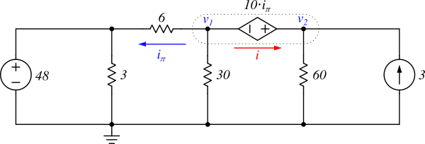
Figure 5: NVM supernode example

In the resistive circuit shown in Figure 5, a current-controlled voltage source is connected between nodes \( v_1 \) and \( v_2 \). To apply KCL at each node, we assume a current \( i \) flowing between the two nodes (as indicated by the red arrow in the figure).

Applying KCL at node \( v_1 \) gives the following equation:

\begin{equation} i_\pi + \frac{v_1}{30} + i = 0 \tag{2.8} \label{eq:ex3_kcl1} \end{equation}

The KCL equation at node \( v_2 \) is:

\begin{equation} -i + \frac{v_2}{60} -3 = 0 \tag{2.9} \label{eq:ex3_kcl2} \end{equation}

By eliminating the shared variable \( i \) from equations~(\ref{eq:ex3_kcl1}) and (\ref{eq:ex3_kcl2}), we get:

\begin{equation} i_\pi + \frac{v_1}{30}+\frac{v_2}{60} -3 = 0 \tag{2.10} \label{eq:ex3_kcl_sn} \end{equation}

Equation~(\ref{eq:ex3_kcl_sn}) is obtained by combining nodes \( v_1 \) and \( v_2 \) and applying KCL to them as a single supernode. This corresponds to summing all four branch currents entering and leaving the dashed supernode in Figure~\ref{fig:ex3}. It clearly demonstrates that when an ideal voltage source connects two nodes, those nodes can be grouped together and treated as a supernode for KCL analysis.

However, by merging two nodes into one supernode, one equation is lost, resulting in fewer equations than unknowns. Fortunately, an additional constraint can be found from within the supernode itself. In this circuit, the voltage of the dependent source inside the supernode is equal to \( v_2 - v_1 \), which yields the following equation:

\begin{equation} v_2 - v_1 = 10\cdot i_\pi \tag{2.11} \label{eq:ex3_inside_sn} \end{equation}

From Figure 5, the control variable \( i_\pi \) of the dependent source is:

\begin{equation} i_\pi = \frac{v_1 - 48}{6} \tag{2.12} \label{eq:ex3_ipi} \end{equation}

Substituting Equation~(\ref{eq:ex3_ipi}) into both (\ref{eq:ex3_kcl_sn}) and (\ref{eq:ex3_inside_sn}), we eliminate \( i_\pi \) and obtain the following system of equations:

\begin{alignat}{3} 16v_1 &&-6v_2 = &&480 \nonumber \\ 12v_1 &&+v_2 = &&660 \tag{2.13} \label{eq:ex3_simul} \end{alignat}

The determinant of the coefficient matrix \( \Delta \) for Equation~(\ref{eq:ex3_simul}) is:

\begin{equation*} \Delta = \left| \begin{array}{rr} 16 & -6 \\ 12 & 1 \end{array} \right| = 16\cdot 1 -(-6)\cdot12 = 88 \end{equation*}

Now we solve for \( v_1 \) and \( v_2 \):

\begin{align*} v_1 &= \frac{1}{\Delta} \left| \begin{array} {rr} 480 & -6 \\ 660 & 1 \end{array} \right|\\ &=\frac{1}{88}(480 \cdot 1 - (-6)\cdot 660) \\ &\approx 50.45\ (V) \\[10pt] v_2 &= \frac{1}{\Delta} \left| \begin{array}{rr} 16 & 480 \\ 12 & 660 \end{array} \right|\\ &=\frac{1}{88}(16 \cdot 660 - 480 \cdot 12)\\ &\approx 54.54\ (V) \end{align*}

Mesh Current Method (MCM)

While the Node Voltage Method (NVM) uses KCL to calculate the voltage at each node, the Mesh Current Method (MCM) uses KVL to calculate the currents flowing through each mesh (a closed loop in the circuit). In NVM, unknown node voltages are used as variables in simultaneous equations. In contrast, MCM uses the current in each mesh as a variable and solves for those using KVL.

MCM with Independent Sources Only

Let’s apply MCM to the circuit in Figure 6 . This circuit has 3 meshes, and the currents are labeled as \( i_1 \), \( i_2 \), and \( i_3 \), all assumed to flow clockwise.

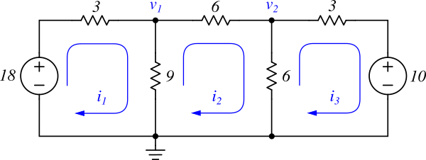
Figure 6: MCM example circuit

First, apply KVL to mesh \( i_1 \). Starting from the GND node (bottom horizontal line in the circuit diagram) and going clockwise, we add the voltage changes one by one:

• The 18V voltage source increases voltage by \( +18 \)
• The \( 3\Omega \) resistor drops \( -3i_1 \)
• The \( 9\Omega \) resistor, shared with mesh \( i_2 \), drops \( -9(i_1 - i_2) \)

The complete KVL equation is:

\begin{equation} 18 - 3i_1 - 9(i_1 - i_2) = 0 \tag{2.14} \label{eq:ex4_kvl1} \end{equation}

Similarly, applying KVL to mesh \( i_2 \) clockwise from GND:

\begin{equation} -9(i_2 - i_1) - 6i_2 - 6(i_2 - i_3) = 0 \tag{2.15} \label{eq:ex4_kvl2} \end{equation}

And for mesh \( i_3 \):

\begin{equation} -6(i_3 - i_2) - 3i_3 - 10 = 0 \tag{2.16} \label{eq:ex4_kvl3} \end{equation}

Combining Equations~(\ref{eq:ex4_kvl1}), (\ref{eq:ex4_kvl2}), and (\ref{eq:ex4_kvl3}), we get the following system:

\begin{alignat}{4} 4i_1 &&-3i_2 &&= &&6 \nonumber\\ 3i_1 &&- 7i_2 && + 2i_3 = &&0 \nonumber\\ &&6i_2 && -9i_3 = &&10 \tag{2.17} \label{eq:ex4_simul} \end{alignat}

The determinant of the coefficient matrix \( \Delta \) is:

\begin{align*} \Delta &= \left| \begin{array}{rrr} 4& -3& 0 \\ 3& -7& 2 \\ 0& 6& -9 \\ \end{array} \right| \\ &= 4\left|\begin{array}{rr}-7&2\\6&-9\end{array}\right| -(-3)\left|\begin{array}{rr}3&2\\0&-9\end{array}\right| +0\left|\begin{array}{rr}3&-7\\0&6\end{array}\right| \\ &=4\cdot(63-12)+3\cdot(-27)\\ &=123 \end{align*}

Now compute \( i_1 \), \( i_2 \), and \( i_3 \):

\begin{align*} i_1 &= \frac{1}{\Delta}\left| \begin{array}{rrr} 6& -3& 0 \\ 0& -7& 2 \\ 10& 6& -9 \\ \end{array} \right| \\ &=\frac{1}{123}(6\cdot(63-12) +3\cdot(-20)) \\ &= 2 \ (A)\\[10pt] i_2 &= \frac{1}{\Delta}\left| \begin{array}{rrr} 4& 6& 0 \\ 3& 0& 2 \\ 0& 10& -9 \\ \end{array} \right| \\ &=\frac{1}{123}(4\cdot(-20) -6\cdot(-27)) \\ &= \frac{2}{3} \approx 0.67\ (A)\\[10pt] i_3 &= \frac{1}{\Delta}\left| \begin{array}{rrr} 4& -3& 6 \\ 3& -7& 0 \\ 0& 6& 10 \\ \end{array} \right| \\ &=\frac{1}{123}(4\cdot(-70) +3\cdot30+6\cdot18) \\ &= -\frac{2}{3} \approx -0.67\ (A) \end{align*}

Finally, using Ohm’s Law, the node voltages \( v_1 \) and \( v_2 \) can be calculated as:

\begin{align*} v_1 &= 9\cdot(i_1 - i_2) \\ &= 9\cdot\left(2-\frac{2}{3}\right) \\ &= 12\ (V) \\[10pt] v_2 &= 6\cdot(i_2 - i_3) \\ &= 6\cdot\left(\frac{2}{3} -(-\frac{2}{3})\right) \\& = 8\ (V) \end{align*}

MCM with Dependent Sources

When applying MCM, the presence of a dependent source in the circuit also introduces additional variables and equations. The general approach remains the same: apply MCM to calculate mesh currents. The only difference is that some extra conditions must be considered due to the dependent source.

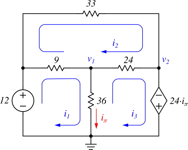
Figure 7: MCM example with a dependent source

To apply MCM to the circuit in Figure 7, we assign mesh current variables \( i_1 \), \( i_2 \), and \( i_3 \), and assume all mesh currents flow in the clockwise direction. This resistive circuit contains a current-controlled voltage source (CCVS), and the control variable \( i_\pi \) is the current flowing through the \( 36\Omega \) resistor. We express this in terms of mesh currents as:

\begin{equation} i_\pi = i_1 - i_3 \tag{2.18} \label{eq:ex5_ipi} \end{equation}

Now, let’s apply KVL to each mesh. First, for mesh \( i_1 \), starting from the GND node and going clockwise:

\begin{equation} 12 - 9(i_1 - i_2) - 36(i_1 - i_3) = 0 \tag{2.19} \label{eq:ex5_kvl1} \end{equation}

Next, for mesh \( i_2 \), starting from node \( v_1 \) and going clockwise:

\begin{equation} -9(i_2 - i_1) - 33i_2 - 24(i_2 - i_3) = 0 \tag{2.20} \label{eq:ex5_kvl2} \end{equation}

Finally, for mesh \( i_3 \), starting from GND and moving clockwise:

\begin{equation} -36(i_3 - i_1) - 24(i_3 - i_2) + 24i_\pi = 0 \tag{2.21} \label{eq:ex5_kvl3} \end{equation}

Substitute Equation~(\ref{eq:ex5_ipi}) into Equation~(\ref{eq:ex5_kvl3}), and simplify all three equations to get the following system:

\begin{alignat}{4} 15 i_1 && -3i_2 && -12i_3 = && 4 \nonumber\\ 3i_1 && - 22i_2 && +8i_3 = && 0 \nonumber\\ 5i_1 && +2i_2 && -7i_3 = && 0 \tag{2.22} \label{eq:ex5_simul} \end{alignat}

The determinant \( \Delta \) of the coefficient matrix is:

\begin{align*} \Delta &=\left| \begin{array}{rrr} 15 & -3 & -12 \\ 3 & -22 & 8 \\ 5 & 2 & -7 \end{array} \right| \\ &= 15(22 \cdot 7 - 8 \cdot 2) - (-3)(3 \cdot (-7) - 8 \cdot 5) -12(3 \cdot 2 + 22 \cdot 5) \\ &= 495 \end{align*}

The values of \( i_1 \), \( i_2 \), and \( i_3 \) are calculated as:

\begin{align*} i_1 &= \frac{1}{\Delta}\left| \begin{array}{rrr} 4 & -3 & -12 \\ 0 & -22 & 8 \\ 0 & 2 & -7 \end{array} \right| \\ &= \frac{4\cdot(22\cdot7 - 8\cdot2)}{495} \\ &= \frac{552}{495} \approx 1.12\ (A) \\[10pt] i_2 &= \frac{1}{\Delta}\left| \begin{array}{rrr} 15 & 4 & -12 \\ 3 & 0 & 8 \\ 5 & 0 & -7 \end{array} \right| \\ &= \frac{-4\cdot(3\cdot(-7) - 8\cdot5)}{495} \\ &= \frac{244}{495} \approx 0.49\ (A)\\[10pt] i_3 &= \frac{1}{\Delta}\left| \begin{array}{rrr} 15 & -3 & 4 \\ 3 & -22 & 0 \\ 5 & 2 & 0 \end{array} \right| \\ &= \frac{4\cdot(3\cdot2 + 22\cdot 5)}{495} \\ &= \frac{464}{495} \approx 0.94\ (A) \end{align*}

The node voltages \( v_1 \) and \( v_2 \) can be easily calculated using Ohm’s Law:

\begin{align*} v_1 &= 36\cdot(i_1 - i_3) \\ &= 36\left(\frac{552}{495} - \frac{464}{495}\right) \\ &= \frac{32}{5} = 6.4\ (V) \\[10pt] v_2 &= -24\cdot(i_1 -i_3) \\ &= -24\left(\frac{552}{495} - \frac{464}{495}\right) \\ &= -\frac{64}{15} \approx -4.27\ (V) \end{align*}

Supermesh

When two meshes in a circuit share an ideal current source on a common branch, they must be treated as a single mesh when applying KVL.

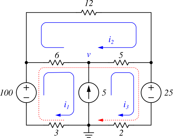
Figure 8: Super Mesh example

Figure 8 shows a resistive circuit used to demonstrate the supermesh concept. To apply MCM, we first assign current variables to each mesh and assume all mesh currents flow clockwise. In the diagram, meshes \( i_2 \) and \( i_3 \) share a \( 5A \) current source on a common branch. Since the voltage across this current source is unknown, we define it as \( v \).

To illustrate the concept of a supermesh, we first apply KVL to mesh \( i_1 \) and \( i_3 \). Starting at the GND node and proceeding clockwise for mesh \( i_1 \):

\begin{equation} -3i_1 + 100 - 6(i_1 - i_2) - v = 0 \tag{2.23} \label{eq:ex6_kvl1} \end{equation}

Likewise, for mesh \( i_3 \), starting at GND:

\begin{equation} v - 5(i_3 - i_2) - 25 - 2i_3 = 0 \tag{2.24} \label{eq:ex6_kvl2} \end{equation}

Eliminating \( v \) from (\ref{eq:ex6_kvl1}) and (\ref{eq:ex6_kvl2}) gives:

\begin{equation} -3i_1 + 100 - 6(i_1 - i_2) - 5(i_3 - i_2) - 25 - 2i_3 = 0 \tag{2.25} \label{eq:ex6_smesh} \end{equation}

Equation~(\ref{eq:ex6_smesh}) is equivalent to applying KVL to the combined supermesh (shown with a red dashed line in Figure 8. This demonstrates that when two meshes share an ideal current source, they must be treated as a single supermesh for the purpose of KVL.

Now apply KVL to mesh \( i_2 \), starting from node \( v \):

\begin{equation} -6(i_2 - i_1) - 12i_2 - 5(i_2 - i_3) = 0 \tag{2.26} \label{eq:ex6_kvl3} \end{equation}

Since there are three unknowns and only two equations so far, we need one more. Within the supermesh, we observe that the shared 5A current source gives:

\begin{equation} i_3 - i_1 = 5 \tag{2.27} \label{eq:ex6_sb} \end{equation}

By substituting \( i_3 \) from (\ref{eq:ex6_sb}) into equations~(\ref{eq:ex6_smesh}) and (\ref{eq:ex6_kvl3}), we obtain the following system:

\begin{alignat}{3} 16i_1 && -11i_2 = && 40 \nonumber\\ 11i_1 && - 23i_2 = && -25 \tag{2.28} \label{eq:ex6_simul} \end{alignat}

The determinant \( \Delta \) of the coefficient matrix is:

\begin{align*} \Delta &=\left| \begin{array}{rr} 16 & -11 \\ 11 & -23 \end{array} \right| \\ &= -16 \cdot 23 + 11 \cdot 11 \\ &= -247 \end{align*}

Now solve for \( i_1 \) and \( i_2 \):

\begin{align*} i_1 &= \frac{1}{\Delta}\left| \begin{array}{rr} 40 & -11 \\ -25 & -23 \end{array} \right| \\ &= \frac{-40 \cdot 23 - 11 \cdot 25}{-247} \\ &= \frac{1195}{247} \approx 4.84\ (A) \\[10pt] i_2 &= \frac{1}{\Delta}\left| \begin{array}{rr} 16 & 40 \\ 11 & -25 \end{array} \right| \\ &= \frac{-16 \cdot 25 - 40 \cdot 11}{-247} \\ &= \frac{840}{247} \approx 3.40\ (A) \end{align*}

Then, from Equation~(\ref{eq:ex6_sb}):

\begin{align*} i_3 &= i_1 + 5 \\ &= \frac{1195}{247} + 5 \approx 9.84\ (A) \end{align*}

Finally, the voltage \( v \) can be found by substituting the values into (\ref{eq:ex6_kvl1}) or (\ref{eq:ex6_kvl2}):

\begin{align*} v_1 &= 100 - 9i_1 + 6i_2 \\ &= 100 - 9\cdot\frac{1195}{247} + 6\cdot\frac{840}{247}\\ &= \frac{18985}{247} \approx76.86 \ (V) \end{align*}

NVM vs. MCM — Which Should You Use?

In fact, both NVM and MCM yield the same results. The question is which is more convenient to use in a given situation. If your goal is to find node voltages, NVM may be more appropriate; if you’re focused on finding branch currents, MCM could be more efficient.

In general:

• If a circuit has many voltage sources, MCM might be easier.
• If it contains many current sources, NVM might be the better choice.

However, this is not a strict rule—it depends heavily on the specific circuit. With more practice and experience analyzing circuits, you'll be able to intuitively choose the method that suits each case best.