SPICE (Simulation Program with Integrated Circuit Emphasis) is an analog electronic circuit simulator. It can be used for anything from board-level circuit design to integrated circuits. It was originally developed at the Electronics Research Laboratory at UC Berkeley in 1973. Since the development of Berkeley SPICE stopped at version 3f5 in 1993, many improved descendants have been released by various vendors.
There are many SPICE variants available, including HSPICE, PSPICE, NGSPICE, LTSPICE, and SPICE OPUS. I chose NGSPICE primarily because it is free and offers good compatibility with KiCAD, which is my main circuit design tool. HSPICE and PSPICE are industry standards, but they are far too expensive for a hobbyist like me. LTSPICE is limited to Windows OS, and I prefer to stick with Linux, where scripting and batch simulations are much more flexible.
How to run NGSPICE?
NGSPICE is essentially a command-line tool, meaning most operations are performed by typing commands and working with text files in a shell environment. There are some GUI integrations available, such as in KiCAD or Qucs-S. You may be tempted to use a GUI at first because it looks easier, but eventually, you'll find yourself returning to the command-line interface for its greater flexibility and wider range of options. In fact, the GUI isn’t very useful unless you understand how things work in command-line mode, and you may even find GUI tools less convenient by comparison. Most people take a hybrid approach—generating netlists using KiCAD or Qucs-S and then including them in an input file for command-line simulation. Therefore, learning NGSPICE the original, command-line way is essential.
Once NGSPICE is installed, typing ngspice at the shell prompt will launch the interactive mode. From there, you can source your input file like this:
% > ngspice
*****************************************
some messages ...
*****************************************
ngspice 1 -> source input_file.cir
Once you're in interactive mode, you can issue various simulation and output requests. You can interactively test and retrieve results from the circuit described in your input file. However, my preferred way to run simulations is to prepare the input file with all the control statements included, and then execute it like this:
% > ngspice input_file.cir
This approach runs the simulation all at once. You can either enter interactive mode after the run or exit back to the shell automatically—depending on how the control statements are written in input_file.cir. You can even run batch simulations using NGSPICE’s control features or shell scripts.
Input File
An input file is used in SPICE simulations. It contains a circuit description—called a SPICE netlist—and control commands. The control block includes analysis settings, output configurations, and basic flow controls.
The typical structure of an input file looks like this:
.title “Simulation Title”

* netlist
* subcircuits
* models

.control
* analysis requests and output controls
.endc

.END
SPICE input files are not case-sensitive. Whether you use uppercase or lowercase makes no functional difference, though it can improve readability. Any line starting with an asterisk (*) is treated as a comment. The first line must contain a title or a comment—leaving it blank will cause an error and make the simulation fail.
NGSPICE supports HSPICE-style syntax, but putting all control statements inside a .control and .endc block gives you more flexibility. You can use all native NGSPICE features within the control block. Finally, don’t forget to place .end at the very end of the file.
SPICE Netlist
A SPICE netlist is a plain ASCII text file that describes a circuit. It specifies how the elements are connected to each other—essentially a textual representation of a circuit diagram. The format for describing an element connection is as follows:
element_name <connected_nodes> <element_value or model_name> <optional_parameters>
The element name must start with a specific letter that corresponds to each type of electrical component. Below are some of the most commonly used letters for SPICE netlist elements:
| First Letter | Element Type | Example |
| R | Resistor | Rout out 0 1K |
| L | Inductor | L12 vin node_1 12M |
| C | Capacitor | C10 3 0 1u |
| D | Diode | Dmod in GND 1N4001 Area=3.0 IC=0.2 |
| Q | BJT | Q1 nC nB nE QMOD IC=0.5 |
| M | MOSFET | M0 nD nG nS nb MOSN L=5u W=2u |
| V | Independent Voltage Source | VCC PWR GND DC 15 VIN N1 N2 0.001 AC 1 SIN(0 1 1MEG) |
| I | Independent Current Source | ISRC 23 21 AC 0.3333 |
| E | VCVS (Voltage-Controlled Voltage Source) | Evc0 n1 n2 ref+ ref- 2M |
| F | CCCS (Current-Controlled Current Source) | FDRV n1 n2 VSEN 5 * VSEN is the name of a voltage source |
| G | VCCS (Voltage-Controlled Current Source) | GOUT 2 0 in 0 2M |
| H | CCVS (Current-Controlled Voltage Source) | HX0 5 17 VZ 0 0.5K |
| X | Subcircuits |
Xop in1 in2 out opamp_1 .subckt opamp_1 plus minus output |
Any string—numbers or text—can be used as node names, but 0 is reserved as the global ground. For voltage-controlled dependent sources like VCVS and VCCS, reference nodes come immediately after the connection nodes. For current-controlled dependent sources like CCCS and CCVS, you must specify the name of the independent voltage source where the reference current is sensed.
In SPICE, the only way to measure current is through an independent voltage source. So, whenever you want to measure the current in a branch, place a zero-volt voltage source in that branch.
Let’s look at an example:
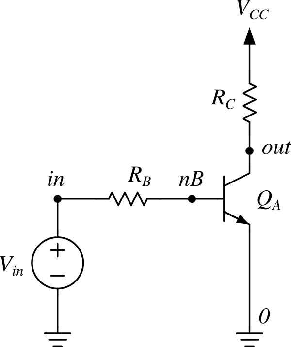
Fig 1. A BJT test circuit
The following is the netlist corresponding to the circuit in Fig. 1:
.global vcc
vcc vcc 0 dc 10
vin in 0 dc 1.7
rb in nb 100k
rc vcc out 5k
qa out nb 0 model_name
Everything should be self-explanatory. The line .global vcc makes the vcc node globally accessible, meaning it can be referenced from anywhere in the circuit. As shown in Fig. 1, the ground node is represented by 0, which is the global ground.
The BJT element qa requires a model name rather than a simple value. There are several ways to define and assign models to active devices, which we’ll cover next.
Applying Models
You can use models provided by NGSPICE. These are general-purpose, minimal models based on various modeling methods and typical application scenarios. For device-specific simulations, however, it's better to download models directly from the manufacturer’s website. Manufacturer-supplied models are typically more accurate and realistic.
That said, when modeling something like a transmission line to mimic a copper trace on a PCB, NGSPICE’s built-in models can still be used effectively—if you choose appropriate parameters, you can achieve reasonably realistic results.
.title The first simulation
*** first_sim.cir

*** Netlist starts here
.global vcc
vcc vcc 0 dc 10
vin in 0 dc 1.7
rb in nb 100k
rc vcc out 5k
qa out nb 0 QMOD
.model QMOD NPN level=1 BF=90

*** Control block starts here
.control
op
print v(out)
.endc

.end
In the example above, a level-1 NGSPICE model is applied to the netlist from Fig. 1, and a simple control block is included. In the .model statement, QMOD is the model name. You can name it anything you like, but it must match the model name used in the qa element line. NPN is the transistor type, and BF=90 sets the forward beta (gain) parameter for the BJT.
The control block includes a single analysis command. The op command tells the simulator to calculate the quiescent (DC operating) point of the circuit. The print command then outputs the voltage at the out node.
Save this as a file named first_sim.cir and run it using the command ngspice first_sim.cir. This will launch interactive mode, and the result will be printed right above the first prompt, like this:
...
No. of Data Rows : 1
v(out) = 5.361446e+00

ngspice 1 -> _
Generating Signals
For transient analysis, you’ll need to generate time-varying signals—such as sine waves, square waves, pulses, etc. Most SPICE simulators provide built-in signal generation commands, which can be added directly to the definition of any independent source.
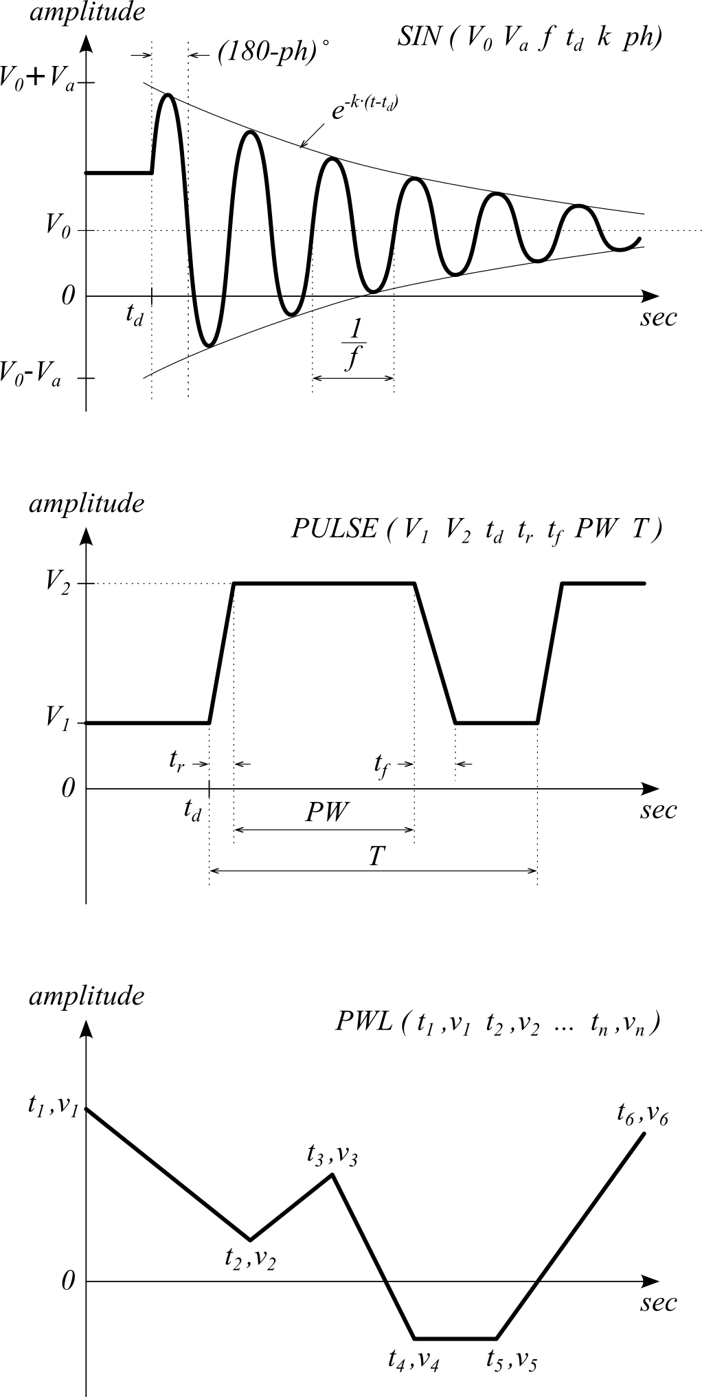
Fig. 2. SPICE signal generation commands
Let’s attach a sine wave signal generator to the vin node in the netlist from Fig. 1:
.global vcc
vcc vcc 0 dc 10
vin in 0 dc 1.7 ac 1 SIN(1.7 1 10K 0 0)
rb in nb 100k
rc vcc out 5k
qa out nb 0 QMOD
.model QMOD NPN BF=90
In the vin voltage source line above, three types of sources are defined—each for a different kind of analysis:
dc 1.7– used for DC analysis and operating point (OP) calculationac 1– used for AC analysis; here,1is a scaling factor, not a voltage valueSIN(1.7 1 10K 0 0)– used for transient analysis; generates a sine wave with:- DC offset: 1.7V
- Amplitude: 1V
- Frequency: 10 kHz
- No delay, no damping, and no phase shift
Using Subcircuits
A subcircuit is a reusable block of netlist, designed for frequent use in circuits. Subcircuits are similar to functions in programming languages. They help reduce repetitive tasks and save time and effort for circuit designers. Subcircuits are also used to model electronic components such as circuit modules or integrated circuits. For example, instead of using a transistor model directly, you can use a subcircuit to represent an op-amp.
Let’s try creating a subcircuit for the BJT shown in Fig. 1. Although subcircuits are not commonly used for single BJTs, this example demonstrates that it is possible.
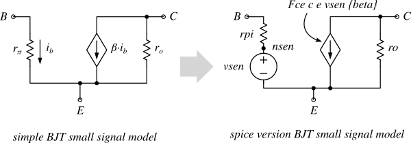
Fig. 3. Simple small-signal BJT model and its SPICE subcircuit equivalent
Fig. 3 shows a simplified small-signal model of a BJT alongside its SPICE subcircuit equivalent. A voltage source vsen is added to sense the reference current for the current-controlled current source (CCCS) Fce. The beta parameter represents the current gain of the BJT.
The input file using this subcircuit looks like the following:
.title The subcircuit example
* first_sim_w_subckt.cir

.global vcc
vcc vcc 0 dc 10
vin in 0 dc 1.7 ac 1 SIN(1.7 1 10K 0 0)
rb in nb 100k
rc vcc out 5k
xqa out nB 0 my_bjt beta=90 rpi=2.5K ro=150K

.subckt my_bjt C B E beta=100 rpi=3K ro=100K
rpi B nSen {rpi}
vsib nSen E 0
Fce C E vsib {beta}
ro C E {ro}
.ends

.control
ac dec 10 1 1e6
let vgain = v(out) / v(in)
meas ac voltage_gain find vgain at=1K
.endc

.end
In the input file above, the subcircuit definition begins with .subckt. The name my_bjt identifies the subcircuit, and C B E are its external terminals. Following the terminal list, you can define parameters (e.g., beta, rpi, ro). The values enclosed in curly braces { } will be replaced with the corresponding parameter values when the subcircuit is instantiated in the netlist. These values can be overridden at the point of use. The name of a subcircuit instance must start with the letter x, which is why xqa is used as the instance name here.
Save the input file as first_sim_w_subckt.cir and run it with NGSPICE:
...
No. of Data Rows : 61
voltage_gain        =  -4.248623e+00
ngspice 1 ->
This matches the hand-calculated result shown below:
\[\begin{align} A_v &= \frac{v_{out}}{v_{in}} \\[10pt] &= -\beta \cdot \frac{R_C \parallel r_o}{R_B + r_\pi} \\[10pt] &= -90 \cdot \frac{150K\Omega \parallel 5K\Omega}{100K\Omega + 2.5K\Omega} \\[10pt] &= -4.248623131 \end{align}\]This subcircuit only works for AC analysis, because the model in Fig. 3 is a small-signal model. Note that the small-signal model only uses ideal sources and resistors, which results in infinite bandwidth, so obtaining frequency response is pointless in this case.
Controls
You can place analysis requests and output controls inside the .control block. NGSPICE also provides programming-like control statements such as while, dowhile, repeat, foreach, and more.
Analysis Requests
To obtain meaningful results from simulation, you must instruct the simulator on what and how to simulate. These instructions are called analysis requests. NGSPICE supports various types of analyses—DC, AC, Transient, Pole-Zero, Distortion, Noise, and more. Some commonly used requests are listed in Table 2.
| Analysis Type | SPICE Syntax |
| Operating Point Analysis | .op |
| DC Transfer Function |
dc srcnam vstart vstop vincr [src2 start2 stop2 incr2]dc VIN 0.25 5.0 0.25dc VDS 0 10 .5 VGS 0 5 1dc VCE 0 10 .25 IB 0 10u 1udc RLoad 1k 2k 100dc TEMP -15 75 5
|
| Small-Signal AC Analysis |
ac (dec | oct | lin) np fstart fstopac dec 10 1 10Kac dec 10 1K 100MEGac lin 100 1 100HZ
|
| Transient Analysis |
tran Tstep Tstop [Tstart [Tmax]] [UIC]tran 1ns 100nstran 1ns 1000ns 500nstran 10ns 1us
|
Output Controls
Output controls define how simulation results are presented or saved. You can print values, plot graphs, or save results to a file for further processing. Here are some commonly used output control formats:
v(n1<,n2>): voltage between node n1 and n2. If n2 is omitted, it's assumed to be ground.I(vsens): current through the independent voltage sourcevsens, flowing from positive to negative terminal.vm(node): magnitude of voltage at node.vp(node): phase of voltage at node.vdb(node): magnitude in decibels (20·log₁₀(vm)).
Using Manufacturer-Provided Models
Let’s run a more realistic simulation using a SPICE model from a semiconductor manufacturer. Download the SPICE model for the 2N2222A NPN BJT from this link. This model is written in the PSPICE format, so you need to enable PSPICE compatibility in NGSPICE.
To do so, create a file named .spiceinit in your home directory and add the following line:
set ngbehavior=ps
Next, rename the downloaded file from 2N2222A.LIB.TXT to 2N2222A.LIB. When you open this file, you will see a line like this:
.MODEL Q2n2222a NPN
...
This line defines the model. To use it in your circuit simulation, simply include the library file in your netlist and reference the model name Q2n2222a in the transistor element line.
.title The First Simulation

*** Netlist starts here
.global vcc
vcc vcc 0 dc 10
vin in 0 dc 1.7 ac 1 SIN(1.7 1 10K 0 0)
rb in nb 100k
rc vcc out 5k
qa out nb 0 Q2n2222a

.inc 2N2222A.LIB

*** Control section starts here
.control
...
.endc

.end
Flow Control
Ngspice provides language-like flow control features. You can use while, dowhile, repeat, foreach, and if-then clauses. Even goto and label are supported, along with continue and break statements.
Let's add some flow control and multiple analysis requests to a netlist using a manufacturer's BJT model to obtain more realistic results. The input file below performs all three types of simulations at once. The repeat control structure is used to run multiple DC sweeps and generate a curve trace for the BJT 2N2222A.
.title The first simulation

*** Netlist starts here
.global vcc
vcc vcc 0 dc 10
vin in 0 dc 1.7 ac 1 SIN(1.7 1 10K 0 0)
rb in nb 100k
rc vcc out 5k
qa out nb 0 Q2n2222a

.inc 2N2222A.LIB

*** Control section starts here
.control
set xbrushwidth=3
let vinn = 0.7
repeat 5
  alter vin $&vinn
  dc vcc 0 20 10m
  let vinn = vinn + 0.1
end
plot (-dc1.I(vcc)) (-dc2.I(vcc)) (-dc3.I(vcc)) (-dc4.I(vcc)) (-dc5.I(vcc))
reset
tran 10n 500u
plot v(in) v(out)
reset
ac dec 10 1 1e6
set units=degrees
plot db(out)
plot ph(out)
.endc

.end
In the input file above, the DC sweep is repeated 5 times, incrementing the vin value by 0.1 V for each run. The negative sign in I(vcc) is necessary because the collector current flows out of the Vcc source, and ngspice defines positive current as flowing into the positive terminal.
After running the five DC analyses, the resulting data groups dc1, dc2, … dc5 can be accessed for plotting. You can run different types of analysis in sequence by using the reset command between simulations to clear the previous state.
Simulation Results

Fig 4. DC sweep simulation for five different vin voltages

Fig 5. Waveforms from transient analysis

Fig 6. Bode plot – gain (dB) vs. frequency (log scale)

Fig 7. Bode plot – phase (degrees) vs. frequency (log scale)
Note: The default NGSPICE plots are fairly basic and limited in interactivity. For better visualization and customization, you can use GNUplot.
Using Gnuplot
Gnuplot is a widely used plotting application. To use Gnuplot, replace the plot command with the gnuplot command. One additional argument is required.
.control
…
reset
ac dec 10 1 1e6
set units=degrees
gnuplot ac_sim db(out) ph(out)
exit
.endc
With NGSPICE’s built-in plotting, all plots disappear once you exit the interactive mode. In contrast, Gnuplot retains the plots even after exiting. You can add the exit command to leave interactive mode after the simulation completes. Another benefit is that the gnuplot command automatically generates a plot control file ac_sim.plt and a data file ac_sim.data. You can modify the .plt file to enhance the plot’s appearance. Keeping these files allows you to redraw the plots anytime. Below is the modified ac_sim.plt file for a dual plot with better labeling. Fig. 8 shows the resulting output.
# ac_sim.plt
# generated by: gnuplot ac_sim db(out) ph(out)
# in the input file "first_sim.cir"

...(omitted)

# The original plot is commented out:
# plot 'ac_sim.data' using 1:2 with lines lw 3 title "db(out)",\
#      'ac_sim.data' using 3:4 with lines lw 3 title "ph(out)"

# Modified for multi-plot
set multiplot
set size 1, 0.5
set origin 0, 0.5
set yrange [0:20]
set ylabel "gain, dB"
set title "AC Analysis - Gain"
plot 'ac_sim.data' using 1:2 with lines lw 3 lt rgb "blue" title "db(out)"
set origin 0, 0
set yrange [0:180]
set ylabel "phase, degrees"
set title "AC Analysis - Phase"
plot 'ac_sim.data' using 3:4 with lines lw 3 lt rgb "red" title "ph(out)"
unset multiplot
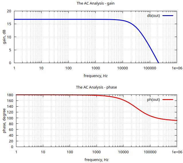
Fig. 8. Output from Gnuplot
Using Gtk Analog Wave Viewer (gaw)
If you're looking for something like Awaves that comes with HSPICE, you can try gaw. While Awaves is more powerful, it’s not a free tool. gaw allows you to use cursor lines to inspect values at each point on the graph, and you can create as many panels as you need. To use gaw, you must first write the simulation data to a file.
.control
set xbrushwidth=3
let vinn = 0.7
repeat 5
  alter vin $&vinn
  dc vcc 0 20 10mv
  let vinn = vinn + 0.1
end
write dc_sim.out (-dc1.I(vcc)) (-dc2.I(vcc)) (-dc3.I(vcc)) (-dc4.I(vcc)) (-dc5.I(vcc))
…
exit
.endc
The usage of the write command is similar to the gnuplot command. Once you run the simulation input file, the example above will save the simulation result into the file dc_sim.out. You can then open this file with the gaw waveform viewer. First, select a panel to draw on, and then choose the signals you want to plot.
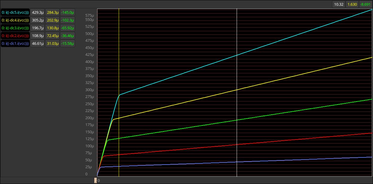
Fig. 9. gaw plot panel
You can use two cursors to measure differences between points, as shown in Fig. 9.
Conclusion
NGSPICE is just as powerful as other SPICE simulators—and in some ways, even better. It’s a very handy tool for hobbyists building precision analog circuits such as amplifiers, RF front-ends, and sensor interfaces. It's also reliable for checking analog front-end and digital I/O interfacing. The usage shown here is only a basic introduction. I hope it provides a useful starting point for hobbyists interested in exploring the world of SPICE.
Even for analog-only applications, NGSPICE offers features like switch models, transmission line models, Monte Carlo simulation, noise sources, non-linear dependent sources, and more. It also supports mixed-mode simulation (analog and digital together). NGSPICE includes support for XSPICE mixed-mode simulation, behavioral modeling, Verilog-A compact device models, digital device models, and digital simulation—opening up a vast range of applications to experiment with.
References
- Ngspice User's Manual – Version 44+. Holger Vogt, Giles Atkinson, Paolo Nenzi, December 29th, 2024.
- NGSPICE Home – Tutorials, introductory videos, downloads, news, and more.
- Gnuplot Homepage – All information and downloads for Gnuplot.
- xschem-gaw GitHub – Download and installation guide for gaw.
Post your comment